Vehicle Simulation Environment
[ VSE Home Page | The 3D environment | Requirements & Installation | Simulation Models | License ]
[ VSE Home Page | The 3D environment | Requirements & Installation | Simulation Models | License ]
As with all extensions to the Java language, the future of Java3D is uncertain. Further development of the Java3D API has been on hold since 2008. If another 3D environment assumes long term dominance, a conversion to that API should not be all that difficult as all VSE graphics dependence is contained within a single package path. One thing to keep in mind - while other 3D graphics packages for Java have come and gone over more than two decades, Java3D is still here and working well on a large variety of hardware and operating systems. This set of libraries has been tested on multiple versions of Linux and Windows, both 32 and 64 bit.
Controls for each environment will depend on the model in use. However, unless the mouse has been remapped in the operating system, the left mouse button will rotate the view while the right mouse button will pan. If a scroll wheel is available, it will control zoom - otherwise, the middle mouse button can be used to zoom in and out.
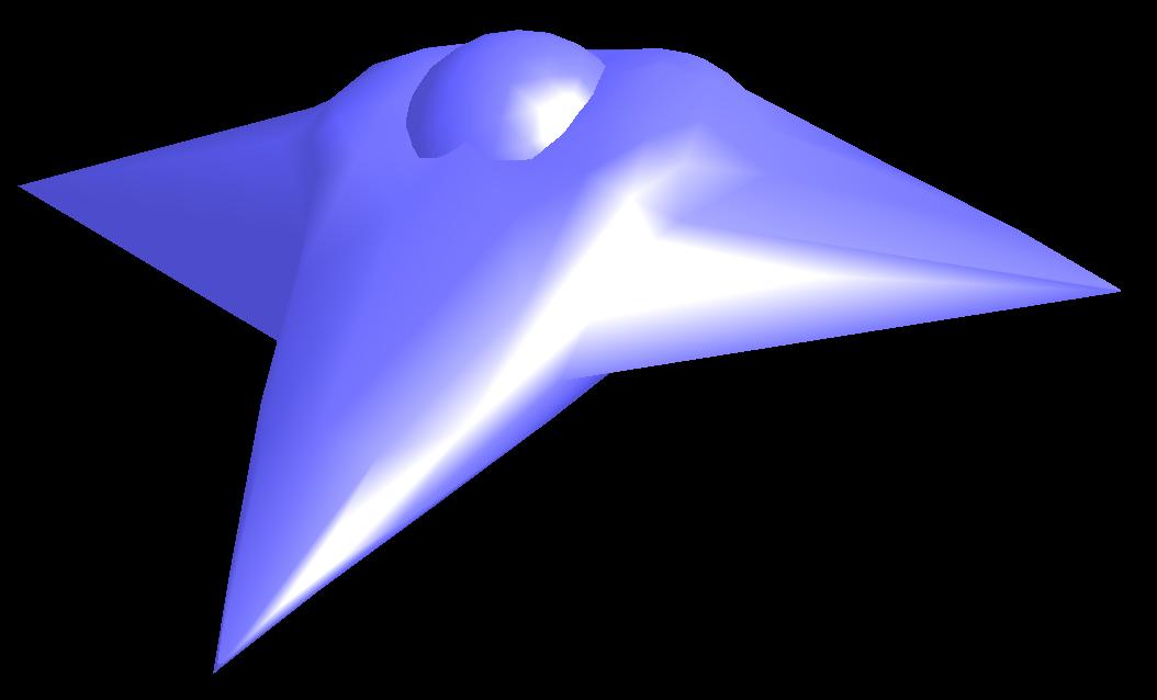
Mesh models have been built with Misfit Model 3D. I am barely competent at using it, so my solid models are very basic....
Java and Java3D installation procedures are best handled by the instructions from their respective download pages. Because installation will differ from one OS to another, I will not attempt to describe it here.
To launch a model in a simulation, it is necessary to install and compile the Vehicle Simulation Environment. Note the full path is "com.motekew.vse".
vseLib-20080930.jarIf the JAR file is not going to be extracted, it is probably easiest to rename or link it to "vseLib.jar" once downloaded. This way, the CLASSPATH environmental variable does not need to be modified each time a new version is downloaded.
Installation of the library involves copying the JAR file to whatever location you like and adding it to your CLASSPATH. How you add it to your CLASSPATH will depend, once again, on the operating system you are using and the environment in which Java is run (command line, shortcut, IDE, etc...). From the command line, in Linux (bash), you would add the following line to your .profile (or similar):
export CLASSPATH=.:/usr/local/javalibs/vseLib.jar:$CLASSPATHThis sets your CLASSPATH environmental variable to include the current directory, the path to vseLib.jar (assuming you copied it to /usr/local/javalibs/), and to include the old CLASSPATH. Sometimes it is easiest to create a simple script that includes a classpath parameter instead of modifying environmental variables (especially under Windows).
Each individual model package follows the same naming convention and is installed in a similar fashion. For example, if the library is installed in /usr/local/javalibs/, and the model is installed in my home directory "kurt", then the update to my CLASSPATH would be:
export
CLASSPATH=.:/usr/local/javalibs/vseLib.jar:/home/kurt/modeling/orbiter.jar:$CLASSPATH
Models, along with classes used to run them in a simulation, are packaged individually as libraries. The primary class in each model package implements an interface needed to start the simulation. This class either needs to be instantiated within a custom application to run, or launched directly with the included RunVSE application (located in RunVSE-YYYYMMDD.jar). This JAR file can either be added to the CLASSPATH, or the RunVSE.class file can be extracted from the jar file with the command:
jar xvf RunVSE.jar RunVSE.classIn addition, utilities than can open .zip files can often open .jar files. Either way, the simulation can be run with the command:
java RunVSE simulation_primary_class_nameFor the above command, if the RunVSE.class was extracted from the RunVSE.jar file, then it is assumed this class resides in the current directory. Otherwise, the RunVSE.jar file needs to be added to your CLASSPATH. Also, the "simulation_primary_class_name" includes the full package path to the model (see models below for the exact syntax to launch each). Note that no class path is needed for the RunVSE application because it was built under the default package.
In Summary, vseLib.jar and RunVSE.jar should be downloaded and added to your CLASSPATH to run any of the models included in this project. All source code is included within each JAR file.
java RunVSE com.motekew.msd3d.MassSpDp3DWhen run, it will ask for the mass, spring constant, and damping properties, along with the initial conditions. The following are reasonable values to start with:
Mass (Kg):  5.0
Spring constant (N/m):  1.0
Damping (N/(m/s)):  0.5
Initial position (m):  7.5
Initial velocity (m/s):  0.0
Start time (s):  0.0
There is only one control for this model - the right arrow will increment a constant force in the positive X direction and the left arrow will increment the force in the negative X direction. This force is set to zero at the start of the simulation. The above initial conditions can be replicated by setting the initial position to zero and incrementing the force with the right arrow 15 times. This results in 7.5 units of force, that will pull the mass 7.5 units along the X-axis. Once the system dampens out, either the up or down arrow will zero the force, causing the mass to be released so it can oscillate about the origin.

When launched, this simulation presents a startup window where the user can enter the gravitational parameter, gravitational scaling radius, and the rotation rate of the central body. The scale factor affects the size of the solid model representing the orbiter. A limited number of gravitational coefficients may also be entered. Check the "Normalized" checkbox when entering normalized coefficients (Kaula normalization is used). No error checking is performed on these values - user beware.
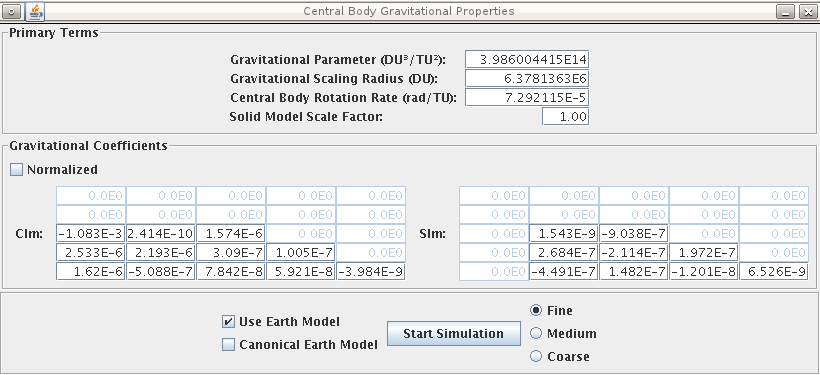
The Use Earth Model option loads real earth values using distance units of meters and time units of seconds. On the display axes, one distance unit is equal to the gravitational scaling radius value. Given the very small integration step size used for the real time simulation, it is recommended that the Canonical Earth Model option be used in conjunction with Use Earth Model.
The display axes calibrations are the corresponding distance units (DU), with 1 DU equal to the gravitational scaling radius of the central body. Time is then in TU, time units. With canonical units, if the central body were an object such as the asteroid 433 Eros, one TU would then be equal to 50.5 minutes. For the earth, one TU is just under 13.5 minutes. The default spacecraft mass is set to 1 with a compatible inertia tensor and control input magnitudes. This results in "real time" attitude rates no matter how TU maps to real world time.
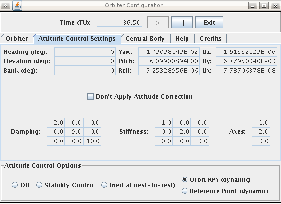
The Orbiter Configuration window, shown below, is comprised of three primary panels. The top section controls execution of the simulation driving the models. The play button (">") moves time forward, while the pause button ("||") halts execution allowing the user to modify settings in the middle tabbed pane section. The bottom panel allows the user to activate different attitude control options during execution.
The Orbiter tab allows the user to adjust orbital parameters and the mass properties of the spacecraft. The user is allowed to create orbits that may result in computational problems. For example, setting the semi-major axis too close to the radius of the central body creates some interesting results that have not been investigated yet. Simply pausing the simulation and changing the orbital elements to something reasonable fixes this.
Four attitude control settings (five, if you count OFF) are available. When the Stability Control button is selected, the control law drives the body axes angular rates to zero by applying appropriate torques derived from a feedback control system. It essentially damps all angular movement. When no user input torques are applied, the system will bring any changes in attitude to a halt. When the user applies torques via the keyboard controls to turn the spacecraft, the attitude control system makes the spacecraft significantly easier to maneuver (at the expense of being a bit more sluggish).
The Inertial (rest-to-rest) attitude control setting orients the spacecraft to a desired heading, elevation, and bank, relative to the inertial X-Y-Z axes. The aerospace sequence is followed for these Euler angles - yaw about the Z-axis, pitch about the new Y-axis, and finally roll about the new X-axis.
The Orbit RPY (dynamic) attitude option orients the spacecraft relative to what is often called the Roll Pitch Yaw frame. It is a local level reference frame in which the Z-axis points towards nadir. The Y-axis is orthogonal to the orbit plane. The X-axis is within the orbit plane, positive in the same direction as the inertial velocity vector. The RPY reference frame is dynamic in nature - the spacecraft must constantly rotate in attempt to maintain the desired attitude. As it is currently implemented, the control system is completely reactionary, with no predictive modeling. Because of this, the actual attitude will slightly lag the desired one depending on how quickly the spacecraft orbits the central body. For example, aligning the spacecraft body axes with the RPY reference frame will result in zero yaw and roll while a slight pitch will always be present. The smaller the semi-major axes, the more noticeable the offset.
The Reference Point options are similar to the Orbit RPY (dynamic) setting except a reference point is used in conjunction with the central body to determine the frame in which attitude is measured. See com.motekew.orbiter.OrbiterSys for more details on the constraints behind these options. The Central Body tab allows the location of the reference point to be set (the default location coincides with the central body).
The Don't Apply Attitude Correction checkbox zeros control system torques within the model. The control system is active, computing yaw, pitch, roll, and corrective torques. However, the corrections are not applied.
Damping controls how aggressively the control law will retard angular motion, while Stiffness affects how much torque is applied given the difference between the desired and current attitudes. More details on these matrices and the control law theory in use can be found in "Rigid-Body Attitude Control Using Rotation Matrices for Continuous, Singularity-Free Control Laws," in the June 2011 IEEE Control Systems Magazine. In the future, more information will be added here regarding the control law gain matrices.
Attitude is specified in Euler angles because they are easy to understand and visualize. Deviations from the desired Euler angles are listed in the Yaw, Pitch, and Roll fields. Uz, Uy, and Ux are the torques applied by the attitude control system (user inputs are not included).
The body axes are aligned such that the X-axis goes through the nose of the spacecraft while the Z-axis is through the top. The Y-axis therefore points out the port "wing". This orientation is slightly unfashionable now days given positive pitch results in a nose-down orientation for aircraft. However, Z should point up. In addition, since the top of an orbiter would generally face towards the central body, falling upside down, positive pitch results in an angle above local level.
No attitude control optimization has been implemented. There are also no limits on the magnitudes of the corrective torques applied by the control system. Attitude quaternions generated by propagation of the model state are passed to the control law. Attitude sensor simulation and attitude determination from sensor models have not yet been implemented.
A new option (not shown - the image will be updated when work on this functionality is complete) is the attitude determination tab ADS. Currently, it allows the user to set the orientation of three simulated star trackers relative to that of the spacecraft body. The single axis angular uncertainty for each sensor may also be set, along with the conewidth dictating the field of view for each sensor. This section is still under development - error checking on limits is very basic at this time.
Upon selecting the Estimate Attitude button, the current time will be displayed along with the true inertial attitude. In addition, the attitude, as determined by the TRIAD algorithm, is displayed. This is used as an initial guess for a very simple weighted least squares estimate of the orbiter attitude.
Additional details on the structure of this model can be found here.
Orbiter is the main class and can be run from the command line with the statement:
java RunVSE com.motekew.orbiter.OrbiterThe Model State Viewer (not pictured here - see Screenshot) is a window that displays the current simulation time, the model state vector, the controls, and the output vector. This is a raw output window generated by the Orbiter model (in contrast to the Orbiter Configuration window that is separate from the model, implemented as part of the simulation). The State Vector is as follows:
X:   X-axis position (DU)
Y:   Y-axis position (DU)
Z:   Z-axis position (DU)
DX:  X-axis velocity (DU/TU)
DY:  Y-axis velocity (DU/TU)
DZ:  Z-axis velocity (DU/TU)
Q0:  Scalar component of Quaternion attitude
QI:  1st vector component of Quaternion attitude
QJ:  2nd vector component of Quaternion attitude
QK:  3rd vector component of Quaternion attitude
P:   Rotation rate about body X-axis (rad/sec)
Q:   Rotation rate about body Y-axis (rad/sec)
R:   Rotation rate about body Z-axis (rad/sec)
Torques and rotations all follow the right hand rule. The Control vector contains only user inputs (no control system inputs):
FX:   X-axis force
FY:   Y-axis force
FZ:   Z-axis force
TX:   Torque about X-axis
TY:   Torque about Y-axis
TZ:   Torque about Z-axis
The Output Vector:
A:      Semi-major axis (DU)
E:      Eccentricity
I:      Inclination (rad)
O:      Right Ascension of the Ascending Node (rad)
W:      Argument of Periapsis (rad)
V:      True Anomaly (rad)
BANK:   Bank (rad)
ELEV:   Elevation (rad)
HEAD:   Heading (rad)
The state vector labels are automatically generated from the Enumerations used to represent them. Bank, elevation, and heading are relative to the RPY reference frame when a central body has been initialized. When a central body is not present, these Euler angles are relative to the inertial X-Y-Z axes. For either case, as stated above, the rotation order follows that of the standard Aerospace sequence.
The values corresponding to A, E, I, O, W, V are the Keplerian orbital elements. They will be non-zero when a central body has been initialized. All angular values displayed in the Model State Viewer are in radians (in contrast to the Orbiter Configuration window).
Screenshot 1 Screenshot 2 Download